A Simple Guide¶

Installation¶

Download zip file from Github
Unzip files at any location, run python setup.py install at the folder where setup.py exists

if you want to modify the code for development, please use python setup.py develop

Run MOC code¶

An example python file to run MOC is provided in /examples/moc. The problem is described as: given the boundaries (upper and lower) and inlet, solve for the flowfield between the upper and lower boundaries.

Import the packages

from aeromoc.moc import MOC2D
from aeromoc.bc import BoundPoints
import numpy as np

Describe the boundary

The boundary of the computation domain are described with a series of points in the class BoundPoints. It is constructed by using add_section. The code below constructs a boundary with two sections. The first section is an 20 degree arc with radius = 6.0 and center located at (0., 8.). The second section is a straight line whose x projection length = 5. and along the tangential direction of the upstream arc.
```
kttau = 20.0
upperwall = BoundPoints()
upperwall.add_section(6 * np.sin(np.linspace(0., np.pi / 180. * kttau, 15)), lambda x: 8. - (6.**2 - x**2)**0.5)
upperwall.add_section(np.linspace(0, 5, 16), lambda x: np.tan(np.pi / 180. * kttau) * x)
```
The boundary points are also the initial points for the character lines, so they are expected to be evenly distributed along the boundaries rather than in x-direction.

For details in boundary conditions, please see Boundary Conditions.
Define the problem

The problem is defined with the object MOC2D. Here, we set up a computional domain where the upper boundary is the wall described in advance, and the lower boundary is a symmetric one.
```
moc = MOC2D()
moc.set_boundary('u', typ='wall', points=upperwall)
moc.set_boundary('l', typ='sym',  y0=0.0)
```
Define the initial line (inlet)

The MOC calculation requires a initial line (in the present program, the left side of computation domain). Here, we use the method in NASA’s code to describe the inlet given the inlet total condition and upstream wall radius.
```
moc.calc_initial_line(n, mode='total', p=2015., t=2726., urUp=9.)
```
For details in inital methods, please see Initial Methods.
Solve for field

The problem is solved with:
```
moc.solve(max_step=100)
```

Show and save the results

moc.plot_field().show()
moc.plot_wall(side='u', var=['p', 'ma', 't'], write_to_file='upper.dat')

For details in postprocess, please see Post-process.

Run nozzle design code¶

An example python file to run MOC is provided in /examples/nozzle. The current code can be used to design the ideal asymmetric SERN proposed by Mo et al. Mo, 2015. The detailed theory can be found in Theory Part

Import the class for designing nozzle

from aeromoc.nozzle import NozzleDesign

Define the problem

Currently, only ideal asymmetric nozzle is available. The nozzle design operating condition are:
- inlet total pressure 200kPa
- inlet total temperature 1393K
- ambient pressure 5kPa
The nozzle design parameters for ideal asymmetric nozzle are:
- asymmetric parameter 0.7, which is defined by $\alpha = \delta_L / \delta_U$
- radius for upper and lower throat upstream contour 3m
(The inlet height is default to be 1m)
```
nz = NozzleDesign('idealAsym', pt=200000, tt=1393, patm=5000, asym=0.7, rup=3., rlow=3.)
```
Solve the design problem
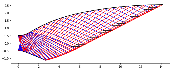
```
nz.solve()
```
The solved nozzle field is like in the figure below:
Apply boundary

To calculate the thickness of boundary layer, the geometry of the convergence section is required. Note that the flow field in convergence section is subsonic, so the field are not solved.
```
nz.gen_conv_section(L=2., yt=0.5, yi=1.)
```
Then the boundary layer thickness is calculated at each contour point, and the corrected contour points are stored.
```
nz.apply_blc()
```
Write contour values

The contour geometry and contour values are written to contour_geometry.dat and contour_values.dat, respectively. The files are in Tecplot format.
```
nz.write_contour()
```
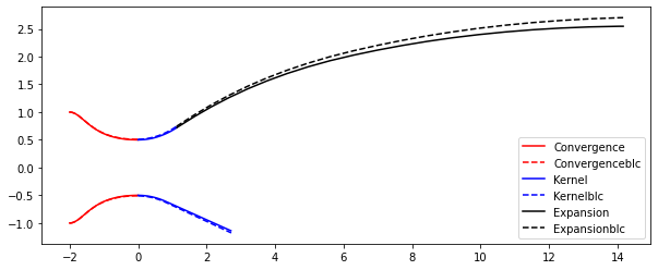
Plot the contour geometries
```
nz.plot_contour()
```
The final plot should be: